Problems in ODE Parameter Fitting

Parameter Identifiability in ODE Models

Fitting experimental data to an ODE model is a deceptively difficult task, especially in the systems biology context. The process itself boils down to finding parameter values that best explain your data, but this is complicated by both parameter identifiability and data sparsity (the latter being ubiquitous in systems biology). Here, we’ll explore how both phenomena can impact parameter fitting results.

Conventional Parameter Optimization

Observe a System and Gather Data

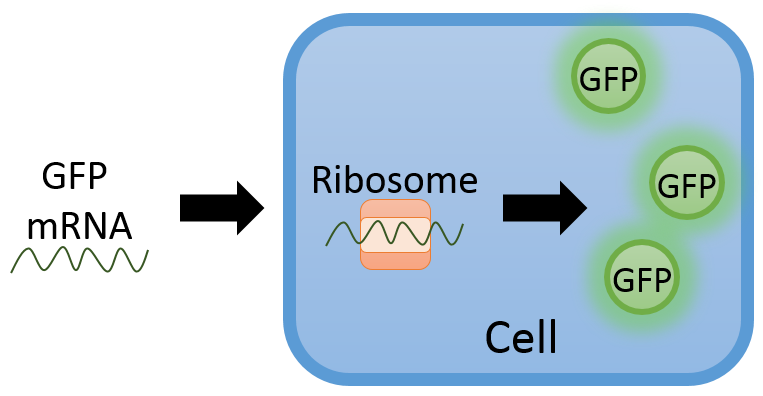
To illustrate a typical procedure for finding parameters in an ODE model, consider the system below where green fluorescent protein (GFP) mRNA is inserted into a cell. The mRNA is translated by the ribosome in the cell to generate the light emitting protein.

Figure_GFP

We can use this system to determine how often GFP mRNA is read by measuring the light intensity given off by the cell. Here is some simulated data showing the dynamics of the GFP (arbitrary units):

Figure_GFP_data

Here we see the light intensity increases and then slowly tapers off, perhaps due to the cell degrading mRNA over time.

Develop a Model to describe Observations

Based on our assumption about mRNA degrading over time, we might develop a two-state ODE model that simulates protein and mRNA dynamics,

\begin{aligned} \frac{d G (t)}{d t} & = k \cdot m (t) - β \cdot G (t) \\ \frac{d m (t)}{d t} & = - τ \cdot m (t) \end{aligned}

subject to the following initial conditions:

\begin{aligned} G (0) & = 0 \\ m (0) & = m_{0} \end{aligned}

The model above consists of four unknown parameters $[k, β, τ, m_{0}]$ with $m_{0}$ being the initial amount of GFP mRNA that entered the cell. Because this is such a simplistic model, we can derive an analytical solution to the system of ODEs:

\begin{aligned} m (t) & = m_{0} e^{- τ t} \\ G (t) & = \frac{k \cdot m_{0}}{β - τ} (e^{- τ t} - e^{- β t}) . \end{aligned}

There is an important note to make here about parameter identifiability. We only have a measurement for $G (t)$ which means $m_{0}$ and $k$ cannot be uniquely determined, but there product ( $m_{0} \cdot k$ ) can be. This is a common occurrence in determining ODE parameter values and is difficult to determine without the analytical solution.

Determine the Best Fit

Using Julia, we can code the ODE model we can run an optimization routine to solve for the parameter values.

#Importing packages
using DifferentialEquations, Random, Plots #Creating ODEs and Plotting
using DiffEqParamEstim, Optim #For finding best fit parameters

###############################################
# Define the ODE Model
###############################################
#Using the fact that m(t) = exp(-τ*t)
    f = function(G,p,t)
        #Assign parameter values
        k, β, τ, m0 = p
        #Write the differential equation
        return k*m0*exp(-τ*t) - β*G
    end

#Parameter values, Initial Conditions, Time (start, end)
    p = [2.0, 0.8, 0.2, 5.0] #true parameter values
    u0 = 0.0
    tspan = (0.0,10.0)
#Contruct the ODE Problem
    prob = ODEProblem(f,u0,tspan,p)
#Solve the ODE problem and plot the solution (Tsit5 is a fancy ODE45)
    sol = solve(prob,Tsit5())
    plot(sol,title="ODE Solution",framestyle=:box,labels=:True)

###############################################
# Generate synthetic data to fit
###############################################

#Set a seed for reproducibility (same stream of random numbers every time)
	Random.seed!(0)
#Create a data set for optimization (adding random normal numbers)
	dataset = [(t,sol(t)+0.2randn()) for t in 0:0.1:10]
#Plot the data on top of the true solution
	scatter!(dataset,framestyle=:box,labels="GFP Data")

###############################################
# Create a cost function and optimize
###############################################

#Cost function
	dataTime = [d[1] for d in dataset] #Collect the time points
	dataValues = [d[2] for d in dataset] #Collect the GFP values
#The cost function needs a few inputs including the ODE problem, ODE solver,
#and L2 error (i.e. sum of squared error)
	cost_function = build_loss_objective(prob,Tsit5(),
                  L2Loss(dataTime,dataValues), maxiters=10000,verbose=false)
#Run the optimizer
	initialGuess = ones(4) #all parameters set to 1
	result = optimize(cost_function, initialGuess) 
#Plot the best parameters found
	probOpt = remake(prob,p=result.minimizer)
	solOpt = solve(probOpt,Tsit5())
	plot!(solOpt,labels=:Optimized,linestyle = :dash)

Figure_GFP_fit

Because the noise added to the data was small, the optimizer was able to get within near perfect agreement of the true solution. How do the optimized parameterized values compare to the true values?

Parameters	True	Initial	Optimized
k	2.0	1.0	2.91
β	0.8	1.0	0.19
τ	0.2	1.0	0.81
$m_{0}$	5.0	1.0	3.45

As expected, the optimized values do not match the true values despite the good fit. The product ( $m_{0} \cdot k$ ) was preserved at a value of 10 and it even looks like the $β$ and $τ$ parameters are non-identifiable as their values are swapped.

This rather simplistic ODE optimization problem demonstrates how much information can be lost when trying to retrieve parameter values and shows how finding the one best parameter can be an ill-posed problem. In upcoming posts we'll investigate techniques for addressing parameter identifiability.