Adding ODEs to CellularPotts.jl

In this blog post, we'll demonstrate how to combine two modeling paradigms to simulate a population of cells dividing.

In the animation above, we see relatively circular blobs that represent cells adhering to one another. The color of each cell relates to the concentration of a theoretical protein X that controls cellular division. As we move forward in time, the concentration of protein X increases to a maximum value of one which triggers the cell to divide into two daughter cells. Protein X randomly distributes between the two new cells after division and two daughter cells also quickly grow to match the size of the other cells.

Let's walk through the code to develop this simulation. There are two characteristics that need to modeled in this simulation, the first being the geometry of each cell and the second being the dynamics of the intracellular proteins.

We begin by loading in both CellularPotts.jl and DifferentialEquations.jl which model the geometry and dynamics respectively.

using CellularPotts, DifferentialEquations

Cellular Potts Modeling

A Cellular Potts Model (CPM) works by defining an array of integer IDs that represent the space where cells are located. Each value in the array corresponds to different objects in the simulation, for example, a value of 0 could represent a point in space with no cell present and a value of 2 could belong to the second cell introduced into the simulation.

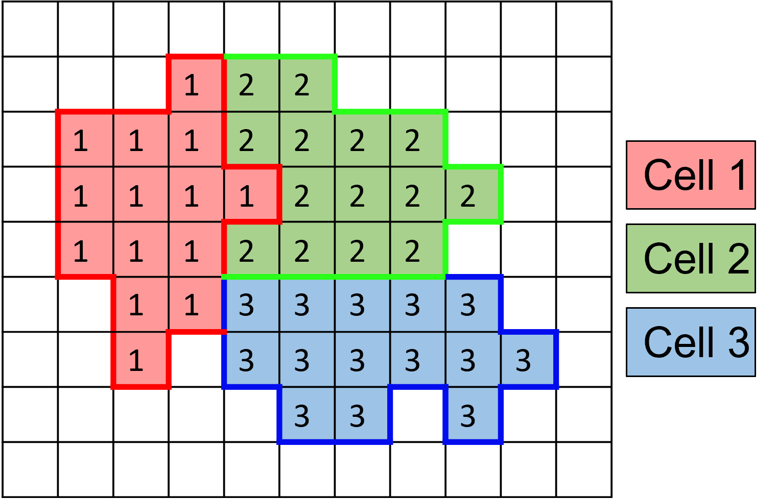
As the CPM steps forward in time, values in the grid are replaced with neighboring values. Penalties (like a cell volume constraint) are added to ensure the simulation mimics desired cell behaviors.

Let's use CellularPotts.jl to create a new model which requires:

• A space for cells to occupy
• A table that summarizes the cells we want to initialize
• A list of penalties to promote desired cell behaviors

The space we will use is a 200×200 grid that defaults to periodic boundary conditions

space = CellSpace(200,200)
200×200 Periodic 4-Neighbor CellSpace{Int64,2}

Next we need to initialize what cells we want in the model.

initialCellState = CellState(:Epithelial, 200, 1, positions = size(space) .÷ 2)

┌────────────┬─────────┬─────────┬─────────┬────────────────┬────────────┬───────────────────┬─────────────────────┐
│      names │ cellIDs │ typeIDs │ volumes │ desiredVolumes │ perimeters │ desiredPerimeters │           positions │
│     Symbol │   Int64 │   Int64 │   Int64 │          Int64 │      Int64 │             Int64 │ Tuple{Int64, Int64} │
├────────────┼─────────┼─────────┼─────────┼────────────────┼────────────┼───────────────────┼─────────────────────┤
│     Medium │       0 │       0 │       0 │              0 │          0 │                 0 │          (100, 100) │
│ Epithelial │       1 │       1 │       0 │            200 │          0 │               168 │          (100, 100) │
└────────────┴─────────┴─────────┴─────────┴────────────────┴────────────┴───────────────────┴─────────────────────┘

Here we define one cell type (Epithelial) which has a desired area of 200 units and we only want 1 to start.

Each row in the table CellTable() represents a cell and each column lists a property given to that cell. Other information, like the column's type, is also provided.

The first row will always show properties for "Medium", the name given to grid locations without a cell type. Most values related to Medium are either default or missing altogether. Here we see our one epithelial cell has a desired volume of 200 and perimeter of 168 which is the minimal perimeter penalty calculated from the desired volume.

Additional properties can be added to our cells using the addcellproperty function. In this model we can provide a special property called positions to place our single cell in the middle of the space.

Now that we have a space and a cell to fill it with, we need to provide a list of model penalties. Here we only include an AdhesionPenalty which encourages grid locations with the same cell type to stick together and a VolumePenalty which penalizes cells that deviate from their desired volume.

penalties = [
    AdhesionPenalty([0 20;
                     20 0]),
    VolumePenalty([5])
    ]

AdhesionPenalty requires a symmetric matrix J where J[n,m] gives the adhesion penalty for cells with types n and m. In this model we penalize Epithelial cell locations adjacent to Medium. The VolumePenalty needs a vector of scaling factors (one for each cell type) that either increase or decrease the volume penalty contribution to the overall penalty. The scaling factor for :Medium is automatically set to zero.

Now we can take these three objects and create a Cellular Potts Model object.

cpm = CellPotts(space, initialCellState, penalties)

Cell Potts Model:
Grid: 200×200
Cell Counts: [Epithelial → 1] [Total → 1]
Model Penalties: Adhesion Volume
Temperature: 20.0
Steps: 0

Connecting Cellular Potts and Differential Equations

This simulation actually extends an example from the DifferentialEquations.jl documentation describing a growing cell population, so much of the code has been taken from this example.

Currently by default CellularPotts models to not record states as they change overtime to increase computational speed. To have the model record past states we can toggle the appropriate keyword.

cpm.record = true;

As Protein X evolves over time for each cell, the CPM model also needs to step forward in time to try and minimize its energy. To facilitate this, we can use the callback feature from DifferentialEquations.jl. Here specifically we use the PeriodicCallback function which will stop the ODE solve at regular time intervals and run some other function for us (Here it will be the ModelStep! function).

function cpmUpdate!(integrator, cpm)
    ModelStep!(cpm)
end

cpmUpdate! (generic function with 1 method)

This timeScale variable below controls how often the callback is triggered. Larger timescales correspond to faster cell movement.

timeScale = 100
pcb = PeriodicCallback(integrator -> cpmUpdate!(integrator, cpm), 1/timeScale);

Differential Equation modeling

The ODE functions are taken directly from the DifferentialEquations example. Each cell is given the following differential equation which models exponential increase in protein X concentration.

$$\frac{\mathrm{d}X}{\mathrm{d}t}=\alpha X$$

const α = 0.3

function f(du,u,p,t)
    for i in eachindex(u)
      du[i] = α*u[i]
    end
end

Also coming from the differential equations example, this callback is triggered whenever Protein X is greater than 1. Basically the cell will divide when when the Protein X concentration is too large.

condition(u,t,integrator) = 1-maximum(u)

function affect!(integrator,cpm)
    u = integrator.u
    resize!(integrator,length(u)+1)
    cellID = findmax(u)[2]
    Θ = rand()
    u[cellID] = Θ
    u[end] = 1-Θ

    #Adding a call to divide the cells in the CPM
    CellDivision!(cpm, cellID-1)
    return nothing
end

This will instantiate the ContinuousCallback triggering cell division

ccb = ContinuousCallback(condition,integrator -> affect!(integrator, cpm));

To pass multiple callbacks, we need to collect them into a set.

callbacks = CallbackSet(pcb, ccb);

Define the ODE model and solve

tspan = (0.0,20.0)
prob = ODEProblem(f,u0,tspan)
sol = solve(prob, Tsit5(), callback=callbacks);

Visualization

We can replicate the plots from the original example

using Plots, Printf, ColorSchemes

Plot the total cell count over time

plot(sol.t,map((x)->length(x),sol[:]),lw=3,
     ylabel="Number of Cells",xlabel="Time",legend=nothing)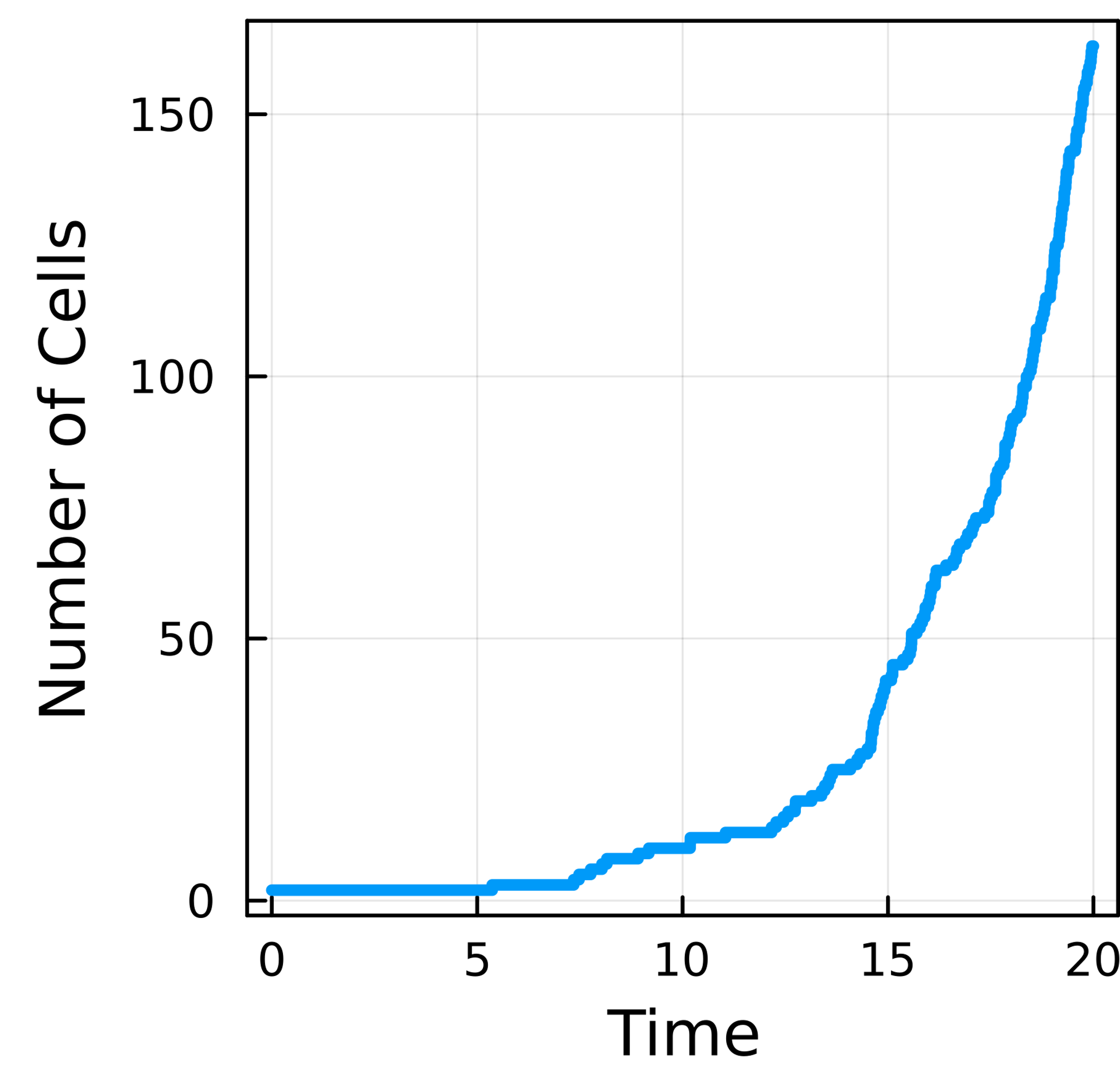

Plot Protein X dynamics for a specific cell

ts = range(0, stop=20, length=100)
plot(ts,map((x)->x[2],sol.(ts)),lw=3, ylabel="Amount of X in Cell 1",xlabel="Time",legend=nothing)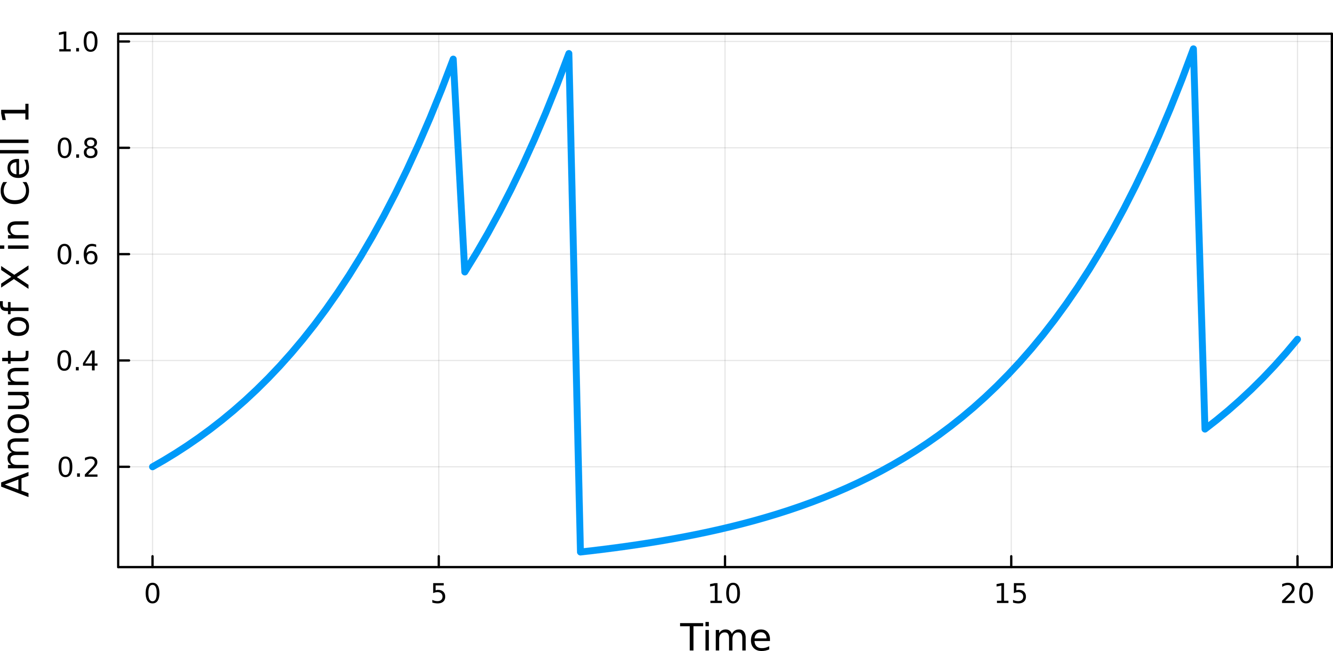

Finally, we can provide the code used to produce the animation we saw at the beginning. I've dropped the first few frames because the first cell takes a while to divide. A link to all the code can be found here

proteinXConc = zeros(size(space))

anim = @animate for t in Iterators.drop(1:cpm.step.stepCounter,5*timeScale)
    currTime = @sprintf "Time: %.2f" t/timeScale

    space = cpm(t).space
    currSol = sol((t+1)/timeScale )

    #Map protein concentrations to space
    for i in CartesianIndices(space.nodeIDs)
        proteinXConc[i] = currSol[space.nodeIDs[i]+1]
    end

    plotObject = heatmap(
        proteinXConc',
        axis=nothing,
        framestyle = :box,
        aspect_ratio=:equal,
        size=(600,600),
        c = cgrad([:grey90, :grey, :gold], [0.1, 0.6, 0.9]),
        clims = (0,1),
        title=currTime,
        titlefontsize = 36,
        xlims=(0.5, size(space.nodeIDs,1)+0.5),
        ylims=(0.5, size(space.nodeIDs,2)+0.5))

    cellborders!(plotObject,space)

    plotObject
end

gif(anim, "BringingODEsToLife.gif", fps = 30)