A New Method for Non-negative Matrix Factorization

What is Non-negative Matrix Factorization?

ODE solution of NMF over time

Non-negative Matrix Factorization (NMF) is an algorithm that decomposes a non-negative matrix $X$ into the product of two non-negative matrices $W$ and $H$. This can be expressed as:

$$X=WH$$

where $X$ is an $n\times m$ matrix, $W$ is $n\times k$, and $H$ is $k\times m$. NMF is useful as a dimension reduction technique because $k$ is typically chosen to be much less than $m$. One way to think about NMF is that each column of $X$ is estimated as linear combinations of the basis vectors in $W$.

$$\left[\begin{array}{c}|\\ x_i\\ |\end{array}\right]=h_{1,i}\left[\begin{array}{c}|\\ w_1\\ |\end{array}\right]+h_{2,i}\left[\begin{array}{c}|\\ w_2\\ |\end{array}\right]+\cdots +h_{k,i}\left[\begin{array}{c}|\\ w_k\\ |\end{array}\right]$$

The goal is to condense information. Instead of dealing with a large number of data columns ($m$ total), we can instead work with a small number of basis vectors ($k$ total).

Multiplicative Update Algorithm

Solving for $W$ and $H$ simultaneously is a non-convex optimization problem (and NP hard); however, solving for one of the matrices while keeping the other constant is convex. Most NMF algorithms take advantage of this by switching back and forth updating $W$ and $H$ until some convergence criteria is met. The first efficient algorithm for NMF performs a simple multiplicative update base on gradient descent:

$${\theta }_{t+1}={\theta }_t-\eta \circ \mathrm{\nabla }D({\theta }_t)$$

where $\theta$ is a some parameter vector (i.e., some point in multidimensional space) being updated and $D$ is the loss function that tells you how well the parameters fit the given model. $\mathrm{\nabla }D$ is the gradient that points to the steepest direction up (we subtract it because we want to find the minimum loss) and $\eta$ is the "learning rate" which scales how large a step we take to the minimum. Note that I'm using the $\circ$ symbol to be explicit about element wise multiplication.

We want to perform gradient decent to optimize both $W$ and $H$:

$$W_{t+1}=W_t-{\eta }_W\circ {\mathrm{\nabla }}_{W}D(W_t)$$$$H_{t+1}=H_t-{\eta }_H\circ {\mathrm{\nabla }}_{H}D(H_t)$$

For NMF a reasonable loss function is:

$$D(X,W,H)=||X-WH|{|}_F^2$$

Where $||\cdot |{|}_F$ is the Frobenius Norm, which we can rewrite in terms of the trace operator.

$$\begin{array}{rlrl}||X-W{H}^{⊺}|{|}_F^2& =tr((X-WH{)}^{⊺}(X-WH))& & \text{Definition of trace for matrix norm}\\ & =tr((X^{⊺}-H^{⊺}{W}^{⊺})(X-WH))& & \text{Transpose property}\\ & =tr(X^{⊺}X-X^{⊺}WH-H^{⊺}{W}^{⊺}X+H^{⊺}{W}^{⊺}WH)& & \text{Expand}\end{array}$$

And then comes the fun part of evaluating the loss function with respect to W and H

$$\begin{array}{rl}{\mathrm{\nabla }}_W||X-WH|{|}^2& ={\mathrm{\nabla }}_W(tr(X^{⊺}X)-tr(X^{⊺}WH)-tr(H^{⊺}{W}^{⊺}X)+tr(H^{⊺}{W}^{⊺}WH))\\ & =0-(H{X}^{⊺}{)}^{⊺}-X{H}^{⊺}+W((H{H}^{⊺}{)}^{⊺}+H{H}^{⊺})\\ & =-2X{H}^{⊺}+2WH{H}^{⊺}\end{array}$$$$\begin{array}{rl}{\mathrm{\nabla }}_H||X-WH|{|}^2& ={\mathrm{\nabla }}_H(tr(X^{⊺}X)-tr(X^{⊺}WH)-tr(H^{⊺}{W}^{⊺}X)+tr(H^{⊺}{W}^{⊺}WH))\\ & =0-(X^{⊺}W{)}^{⊺}-W^{⊺}X+(W^{⊺}W+(W^{⊺}W{)}^{⊺})H\\ & =-2W^{⊺}X+2W^{⊺}WH\end{array}$$

Whew, now we can take these two results and substitute them back into our gradient decent equations for W and H:

$$W_{t+1}=W_t+{\eta }_W\circ (X{H}_t^{⊺}-W_t{H}_t{H}_t^{⊺})$$$$H_{t+1}=H_t+{\eta }_H\circ (W_t^{⊺}X-W_t^{⊺}{W}_t{H}_t)$$

Note that the factor of two was "absorbed" into the learning rate (you could also add a 1/2 factor to the loss function, it doesn't really matter). There is an issue with the equations we've written down so far. They contain negative terms! Luckily we still have to define the learning rate parameters which we can set to anything we like. Lee and Seung proposed defining the learning rates as:

$${\eta }_W=\frac{W}{WH{H}^{⊺}}$$$${\eta }_H=\frac{H}{W^{⊺}WH}$$

which when we substitute into the descent equation gives some nice cancelation:

$$\begin{array}{rl}{W}_{t+1}& =W_t+\left(\frac{W_t}{W_t{H}_t{H}_t^{⊺}}\right)\circ (X{H}_t^{⊺}-W_t{H}_t{H}_t^{⊺})\\ & =W_t+W_t\circ \frac{X{H}_t^{⊺}}{W_t{H}_t{H}_t^{⊺}}-W_t\circ \frac{W_t{H}_t{H}_t^{⊺}}{W_t{H}_t{H}_t^{⊺}}\\ & =W_t\circ \frac{X{H}_t^{⊺}}{W_t{H}_t{H}_t^{⊺}}\end{array}$$$$\begin{array}{rl}{H}_{t+1}& =H_t+\left(\frac{H_t}{W_t^{⊺}{W}_t{H}_t}\right)\circ (W_t^{⊺}X-W_t^{⊺}{W}_t{H}_t)\\ & =H_t+H_t\circ \frac{W_t^{⊺}X}{W_t^{⊺}{W}_t{H}_t}-H_t\circ \frac{W_t^{⊺}{W}_t{H}_t}{W_t^{⊺}{W}_t{H}_t}\\ & =H_t\circ \frac{W_t^{⊺}X}{W_t^{⊺}{W}_t{H}_t}\end{array}$$

And these are the two update rules for NMF:

$$W_{t+1}=W_t\circ \frac{X{H}_t^{⊺}}{W_t{H}_t{H}_t^{⊺}}$$$$H_{t+1}=H_t\circ \frac{W_t^{⊺}X}{W_t^{⊺}{W}_t{H}_t}$$

Essentially you pick two random starting points for $W$ and $H$, then you use these equations to iteratively update the solution until the solution stops changing significantly.

Solving NMF with Ordinary Differential Equations

Let's look back at our gradient decent equation:

$${\theta }_{t+1}={\theta }_t-\eta \circ \mathrm{\nabla }D({\theta }_t)$$

instead of taking discrete steps toward a local minima, we could look at the limit as we take smaller and smaller step sizes:

$$\begin{array}{rlrl}{\theta }_{t+1}& ={\theta }_t-\mathrm{\Delta }t\circ \mathrm{\nabla }D({\theta }_t)& & \text{Set }\eta \text{ to }\mathrm{\Delta }t\\ \underset{\mathrm{\Delta }t\to 0}{lim}\frac{{\theta }_{t+1}-{\theta }_t}{\mathrm{\Delta }t}& =-\mathrm{\nabla }D({\theta }_t)& & \text{Take limit}\\ \frac{d\theta }{dt}& =-\mathrm{\nabla }D({\theta }_t)& & \text{Definition of derivative}\end{array}$$

This approach is known as gradient flow. When applied to NMF, we end up with a system of coupled differential equations:

$$\frac{dW}{dt}=W\circ (\frac{X{H}^{⊺}}{WH{H}^{⊺}}-\mathbb{1})$$$$\frac{dH}{dt}=H\circ (\frac{W^{⊺}X}{W^{⊺}WH}-\mathbb{1})$$

Here I'm trying to be explicit about the fact that we are doing an element-wise multiplication, division, and subtraction. $\mathbb{1}$ represents a matrix of ones with the appropriate size for each equation.

Head-to-Head Comparison

To compare the discrete and continuous versions of these NMF algorithms, I want to focus on overall accuracy as opposed to speed (which will boil down to the number of matrix multiplications performed). I will perform the factorization on the following matrix which defines a circle of random numbers.

using Plots

n,m = (400,500)
k = 40
W0 = rand(n,k)
H0 = rand(k,m)

X = [(x-200)^2+(y-200)^2>50^2 ? rand() : 10*rand() for x in 1:n, y in 1:m]

heatmap(X,clims=(0,10))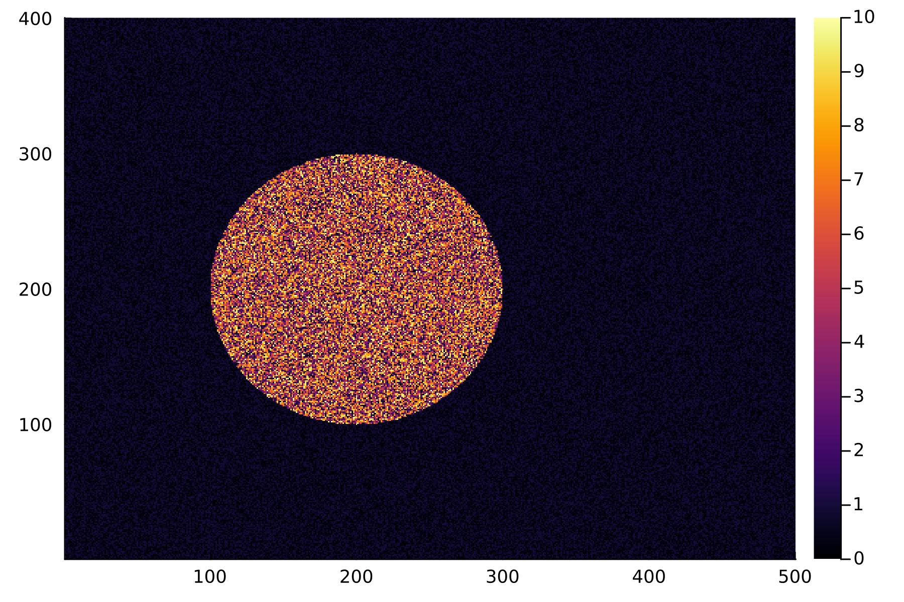

The ODE method is going to automatically choose the step size based on the solver choice. To make a fair comparison, I will run the multiplicative update for the same number of iterations.

ODE Implementation

using LinearAlgebra
using OrdinaryDiffEq
using RecursiveArrayTools

# Define ODEs
function nmf!(du, u, p, t)

    X, WH, XHᵀ, WHHᵀ, WᵀX, WᵀWH = p
    W = u.W
    H = u.H

    mul!(WH,   W,  H)
    mul!(XHᵀ,  X,  H')
    mul!(WHHᵀ, WH, H')
    mul!(WᵀX,  W', X)
    mul!(WᵀWH, W', WH)

    @. du.W = W * (XHᵀ / WHHᵀ - 1)
    @. du.H = H * (WᵀX /WᵀWH  - 1)
end

WH = similar(X)
XHᵀ = similar(W0)
WHHᵀ = similar(W0)
WᵀX = similar(H0)
WᵀWH = similar(H0)

p = (X, WH, XHᵀ, WHHᵀ, WᵀX, WᵀWH)
u0 = NamedArrayPartition((;W=W0,H=H0))
tspan = (0.0, 1000.0)

#Solving
prob = ODEProblem(nmf!, u0, tspan, p)
sol = solve(prob,ROCK4())

I tried a few different ODE solvers and found ROCK4 to be very efficient.

Multiplicative Update Implementation

mutable struct NMFMU{M}
    X::M
    W::M
    H::M
end

nmf = NMFMU(copy(X),copy(W0),copy(H0))

function MU!(nmf::NMFMU)

    nmf.W .= nmf.W .* (nmf.X * nmf.H') ./ (nmf.W * nmf.H * nmf.H')
    nmf.H .= nmf.H .* (nmf.W' * nmf.X) ./ (nmf.W' * nmf.W * nmf.H)

    return nothing
end

This is very inefficient implementation, for an optimized version please use the NMF.jl package.

Loss over Iterations

#error  
loss(X,W,H) = norm(X-W*H) / norm(X)
loss(nmf) = loss(nmf.X, nmf.W, nmf.H)

#ODE
ode = [loss(X,sol[i].W,sol[i].H) for i in eachindex(sol)]
pushfirst!(ode,loss(X,W0,H0))

  
#MU
mu = [loss(X,W0,H0)]

for _ in eachindex(sol)
    MU!(nmf)
    push!(mu,loss(nmf))
end

plot(ode, label="ODE", linewidth=3, xlabel="Iterations", ylabel="Error")
plot!(mu, label="MU", linewidth=3)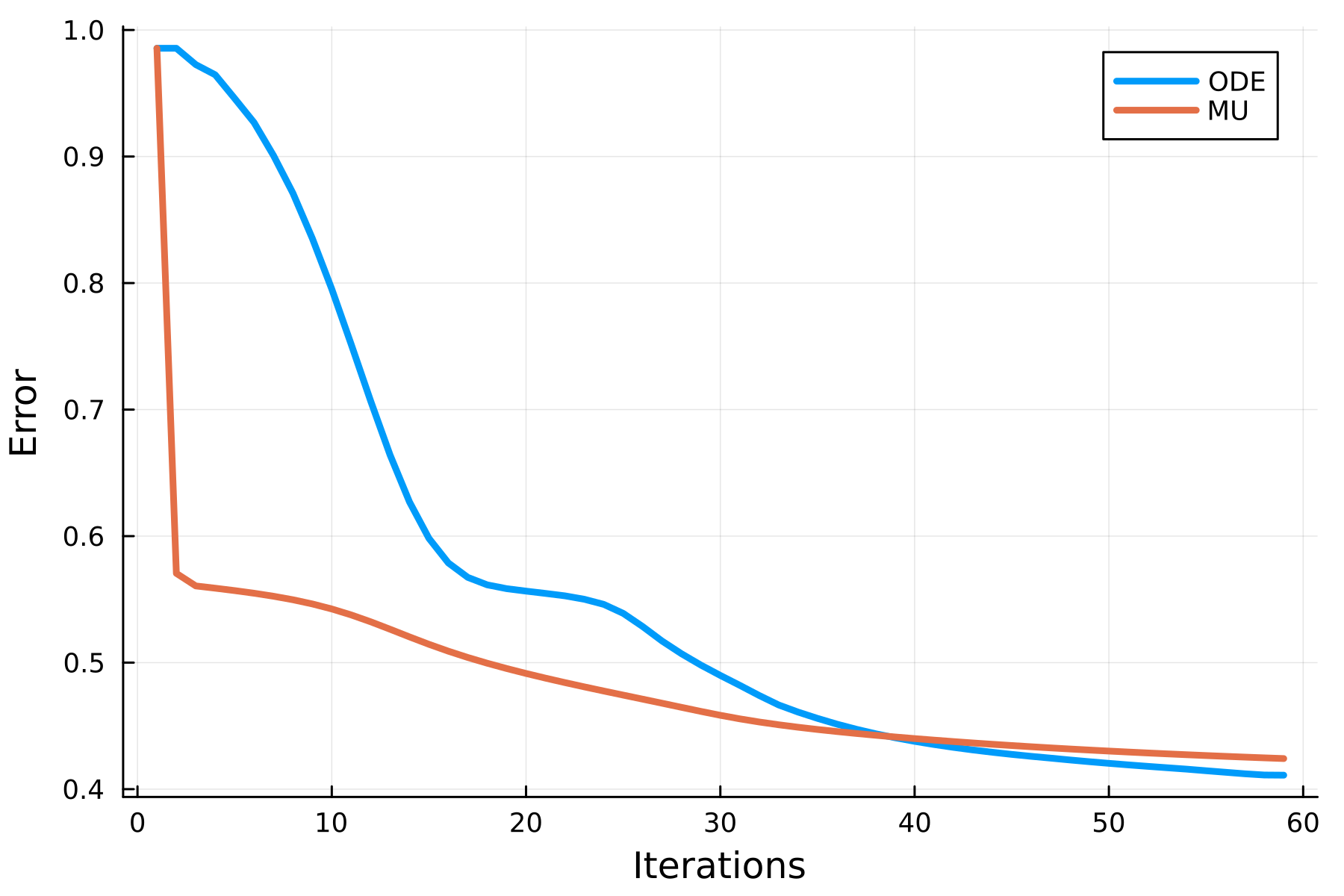

The first thing I notice is the first step each algorithm. MU takes a huge step in the right direction whereas the ODE method is very conservative in its decent. More surprising is that the final solutions are different. At least for this kind of random matrix, the ODE method is able to find a better solution. Maybe MU would eventually end up at the same solution? I've ran these methods for more iterations but this does not seem to be the case.

There are a lot of improvements and variations we can do with this system like accelerated gradient decent, translating more efficient NMF algorithms, and investigating steady state solutions. Hopefully this will lead to better algorithms for NMF!