Hello World

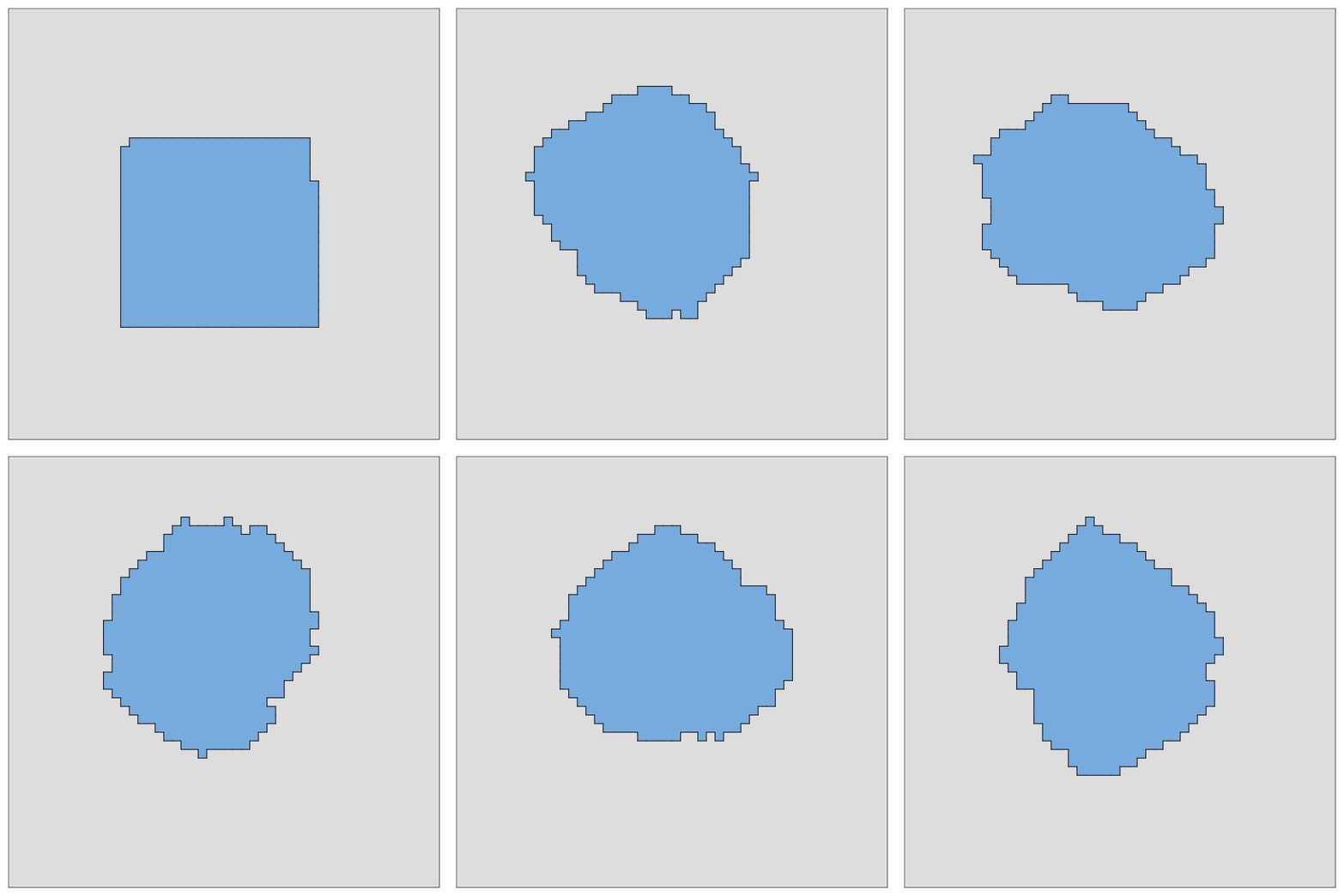
In this example, we'll specify a single stationary cell in the center of the grid.

We start by loading in the CellularPotts.jl package and creating a space where cells can exist.

using CellularPotts

space = CellSpace(50,50; periodic=true, diagonal=true)

50×50 Periodic 8-Neighbor CellSpace{Int64,2}

Here we create a 50 by 50 square grid with periodic boundary conditions where grid locations are connected to their 8 closest neighbors, also called Moore neighbors (4-cell neighborhoods that exclude diagonal neighbors are called Von Neumann). By default, periodic is set to true and diagonal is set to false.

Next we need to initialize a table of cell information to put into this space.

initialCellState = CellState(:Epithelial, 500, 1; positions = (25,25))

┌────────────┬─────────┬─────────┬─────────┬────────────────┬────────────┬───────────────────┬─────────────────────┐
│      names │ cellIDs │ typeIDs │ volumes │ desiredVolumes │ perimeters │ desiredPerimeters │           positions │
│     Symbol │   Int64 │   Int64 │   Int64 │          Int64 │      Int64 │             Int64 │ Tuple{Int64, Int64} │
├────────────┼─────────┼─────────┼─────────┼────────────────┼────────────┼───────────────────┼─────────────────────┤
│     Medium │       0 │       0 │       0 │              0 │          0 │                 0 │            (25, 25) │
│ Epithelial │       1 │       1 │       0 │            500 │          0 │               264 │            (25, 25) │
└────────────┴─────────┴─────────┴─────────┴────────────────┴────────────┴───────────────────┴─────────────────────┘

The CellState() function populates a table detailing the current cell state. The 3 required inputs are:

1. A list of cell types
2. A list of desired cell sizes (volumes)
3. A list of cell counts for each cell type

The inputs are simple in this case. We want one cell type called "Epithelial" with a size of 500 pixels and we want only one of them.

In addition to the 3 required inputs, we can use the optional keyword positions to place the cell at a given location. Because the space we specified is 2D, we provide an x and y coordinate to position the cell in the center.

The table CellState() generates has each row representing a cell and each column listing a property given to that cell. Other information, like the column's type, is also provided. Custom properties can be added with the addcellproperty() function.

The first row will always show properties for "Medium", the name given to grid locations without a cell type. Most values related to Medium are either default or missing altogether. Here we see our one epithelial cell has a desired volume of 500 and perimeter of 264 which is the minimal perimeter penalty calculated from the desired volume.

Now that we have a space and a cell to fill it with, we need to provide a list of model penalties. A number of default penalties exist and you can even create your own custom penalties. Here we only include an AdhesionPenalty which encourages grid locations with the same cell type to stick together and a VolumePenalty which penalizes cells that deviate from their desired volume.

penalties = [
    AdhesionPenalty([0 20;
                     20 0]),
    VolumePenalty([5])
    ]

2-element Vector{Penalty}:
 Adhesion
 Volume

AdhesionPenalty requires a symmetric matrix J where J[n,m] gives the adhesion penalty for cells with types n and m. In this model we penalize Epithelial cell locations adjacent to Medium. The VolumePenalty needs a vector of scaling factors (one for each cell type) that either increase or decrease the volume penalty contribution to the overall penalty. The scaling factor for :Medium is automatically set to zero.

Now we can take these three objects and create a Cellular Potts Model object.

cpm = CellPotts(space, initialCellState, penalties)

Cell Potts Model:
Grid: 50×50
Cell Counts: [Epithelial → 1]
Model Penalties: Adhesion Volume
Temperature: 20.0
Steps: 0

Calling this object gives a quick summary of the model's current state. Note that a "temperature" of 20 is given to the model by default. Higher temperatures allow the model to more likely accept changes that increase the overall penalty (e.g. cells could deviate further from their desired volume). The model object also tracks how many time steps have been performed.

Our model is more ready for simulation! This can be done using the using the ModelStep! function or recorded as a gif using recordCPM

recordCPM("HelloWorld.gif", cpm)

This page was generated using Literate.jl.